Cutter Dawes

An underappreciated fact about large language models (LLMs) is that they are at once two separate things: (i) a representation machine, in which the fundamental objects are features in a geometrically complex latent space; and (ii) a probabilistic model, in which the fundamental objects are logits corresponding to a probability distribution over language. The merging of these two regimes is foundational to LLM capabilities, but how they do so as they process activations layer-by-layer is still poorly understood. Though much progress has been made towards understanding each regime, a significant gap still remains in understanding how they relate with each other. This gap has only widened with the advent of chain of thought (CoT) reasoning, as models build ever more sophisticated representations whose purpose is increasingly disconnected from the immediate next-token logits.

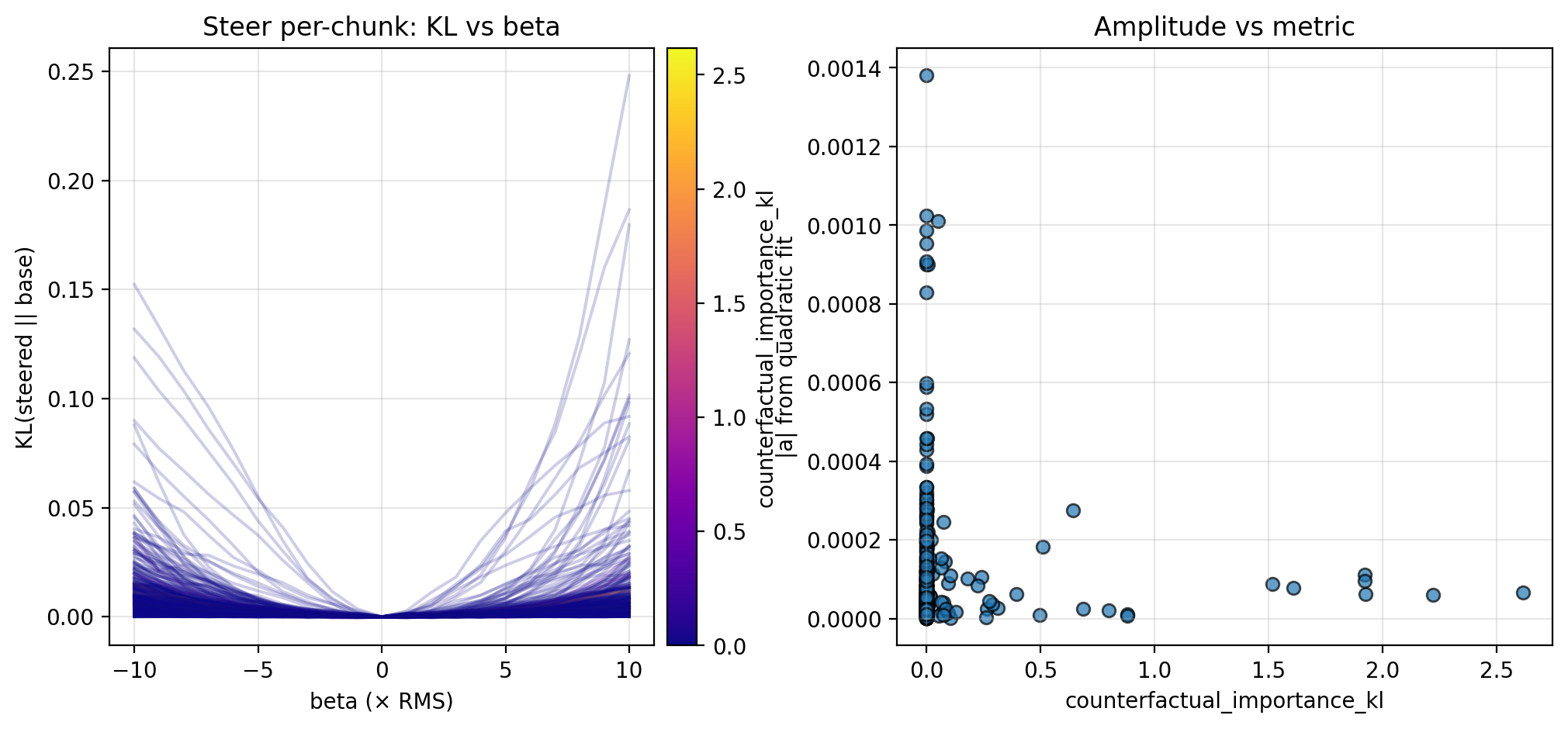
In this post, I hope to contribute towards bridging that gap—to better connect geometric properties of latent space to downstream logits. In particular, I probe the local steepness around latent activations and measure the relationship to probabilistic metrics that measure importance at the logit level. I first generate and annotate responses to the MATH dataset using the same metrics as in the recent “Thought Anchors” paper (Bogdan et al. 2025; henceforth TA), and then I find latent activations corresponding to sentence chunks in the CoTs. Next, I measure local steepness in latent space by steering chunk activations with small magnitudes and measuring the KL divergence between the base and steered logits. I compare these steepness measurements to the metrics in TA; see the figure below for one such result. Notice the inverse relationship between the local steepness (y-axis in scatterplot) and the counterfactual importance (x-axis; one of the probabilistic metrics from TA). This inverse relationship is visible in many of the figures shown in this post: collectively, they suggest that activations in locally flat regions of latent space tend to be more important to downstream computation. These relationships, though preliminary, add to recent indications that geometric properties of latent space play a potentially significant role in the downstream thought process.

Code for this project is available at github.com/cutterdawes/SteeringThoughtAnchors.

1. Related Work

1.1. Representational Regime: Latent Space Geometry

There is a large body of literature investigating the rich structure of LLM representations, whose scope varies from two extremes: (0) individual features or feature groups, and (1) the global geometry that permeates the feature space. At the local feature level, work has identified space and time directions in latent space (Gurnee et al. 2023) and integers represented along a helix (Kantamneni et al. 2025). Pulling back, there has been support for (Jiang et al. 2025) and against (Engels et al. 2024) the linear representation hypothesis (Park et al. 2023). Even more globally, work has studied the extent to which latent representations satisfy the manifold hypothesis (Robinson et al. 2025) as well as connections between intrinsic dimension and generalization (Ruppik et al. 2025).

1.2. Probabilistic Regime: Logit-Level CoT

As reasoning becomes the next frontier of progress in artificial intelligence, it has brought with it a wave of research seeking to understand CoT. In particular, much effort has gone into quantifying how faithful CoT is to the underlying reasoning process (Arcuschin et al. 2025). Recent work (TA) has also found evidence of “thought anchors”, reasoning steps that have outsized importance for downstream steps in the model’s chain of thought. The paper’s core contributions are: (i) chunking thought at the sentence-level, choosing sentences as the atom of analysis for CoT reasoning; and (ii) measuring sentence importance at the probabilistic level by resampling just before each sentence, and measuring the outcomes along similar and dissimilar CoT trajectories. (Significantly, they also poke below the probabilistic regime to observe and ablate attention between sentences, but that is beyond the scope of this post.)

1.3. Bridging the Gap

There has also been an under-appreciated area of research seeking to bridge the representational and probabilistic regimes. This project has become especially urgent given the possibly narrow window of time in which CoT remains legible (Korbak et al. 2025). Previous work includes steering CoT towards certain categories of thinking (Venhoff et al. 2025). There has also been a line of research that dates back multiple years, which explores how metrics in representation space can be connected to downstream logits. In particular, previous work has demonstrated that the Fisher-Rao metric (defined on smooth manifolds whose points are probability distributions) can be pulled back to earlier layers of neural networks to induce a distance on latent representation spaces (Liang et al. 2019, Arvanitidis et al. 2021). It turns out that this metric exactly corresponds to the local KL divergence between the logits induced by latent activations; that is, it produces a correspondence between the activation- and logit-level regimes.

2. Preliminaries

2.1. Reproducing TA

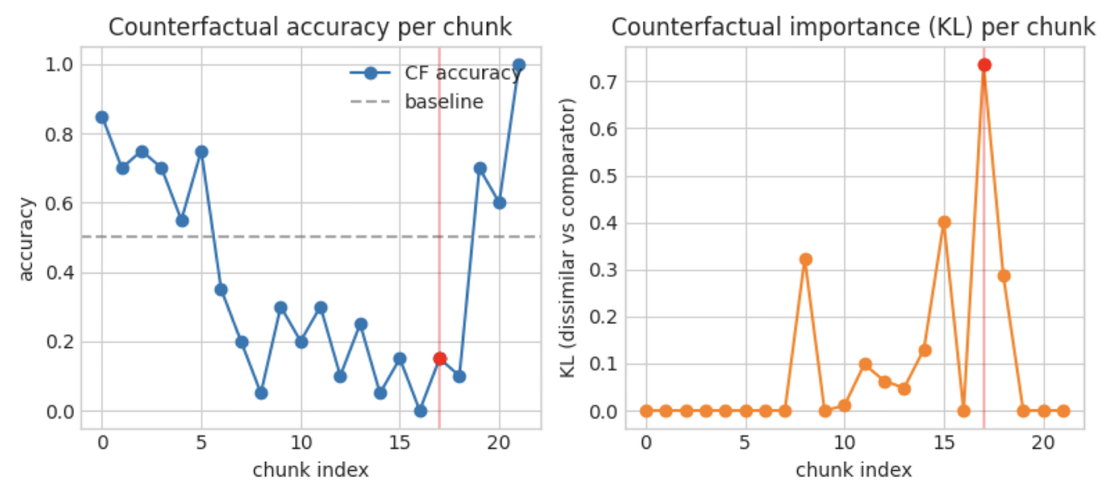
I first reproduce the data generation and annotation procedure in TA, with some minor differences noted below. Using the MATH dataset and the R1-distilled Qwen 1.5B reasoning model, I generate 5 responses each for 100 questions (sampled from MATH Level 2; with CoT token lengths at most 500, followed by a forced answer—this is in contrast to the much-longer CoTs of TA, due to compute restraints). I identify 28 promising examples for which the model obtains 0.2-0.8 accuracy rates. For these 28 examples, I annotate the model’s CoT by breaking into sentence chunks and resampling each chunk 20 times, measuring the same metrics as in TA for each chunk:

1. counterfactual accuracy, the averaged answer accuracy of resampled CoTs;

2. different trajectories fraction, the percentage of resampled CoTs which immediately depart from the original chunk;

3. counterfactual importance, the KL divergence between answer distributions of similar and dissimilar resampled trajectories.

The figure below displays counterfactual accuracy and importance for one example, a la Figure 2 in TA.

2.2. Collecting Chunk Latent Activations

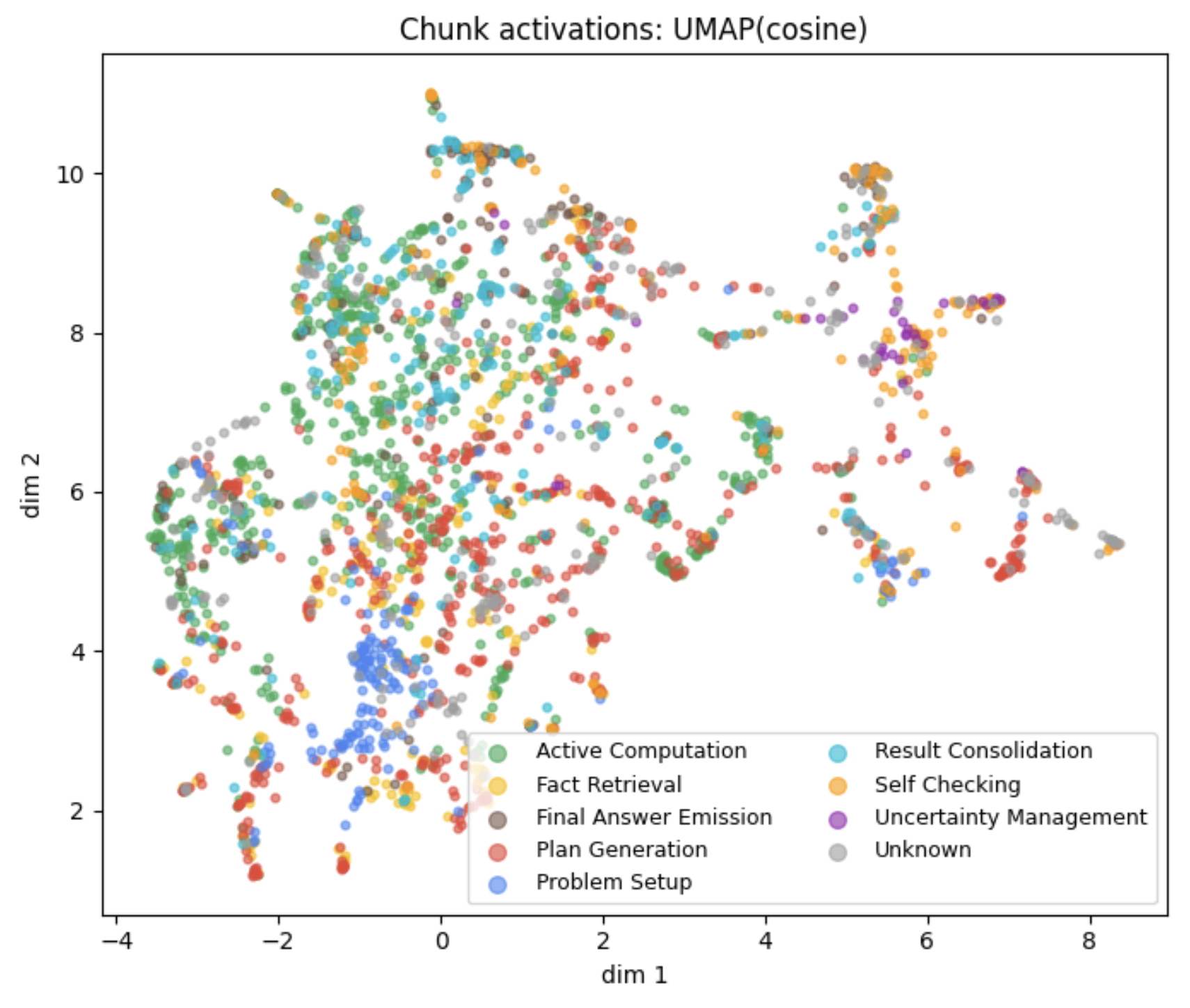
Next, I collect latent activations for chunks in the generated CoTs. For this study, I use activations on layer 24 after some preliminary testing and because it is in the common range of layers used in activation engineering. To obtain chunk-wide activations, I mean-pool the token-level activations in each chunk. In the figure below, I plot the UMAP-projected activations for 100 generated CoTs (totaling 2688 chunks), color-coded by the same categories as used in TA (labelled using Qwen 3B Instruct). Observe that, even in 2 dimensions (reduced from ~1500), chunks cluster by category and suggest intricate latent structure.

3. Experiments

In this study, I investigated possible connections between the local geometry of chunk activations and the probabilistic measurements from TA. To probe this relationship, I steered chunk activations by different vectors with small steering magnitudes (Section 3.1), perturbed chunk activations in random directions to investigate the overall steepness (Section 3.2), and investigated the ratio of steepness between different directions to better understand the steepness’ shape (Section 3.3).

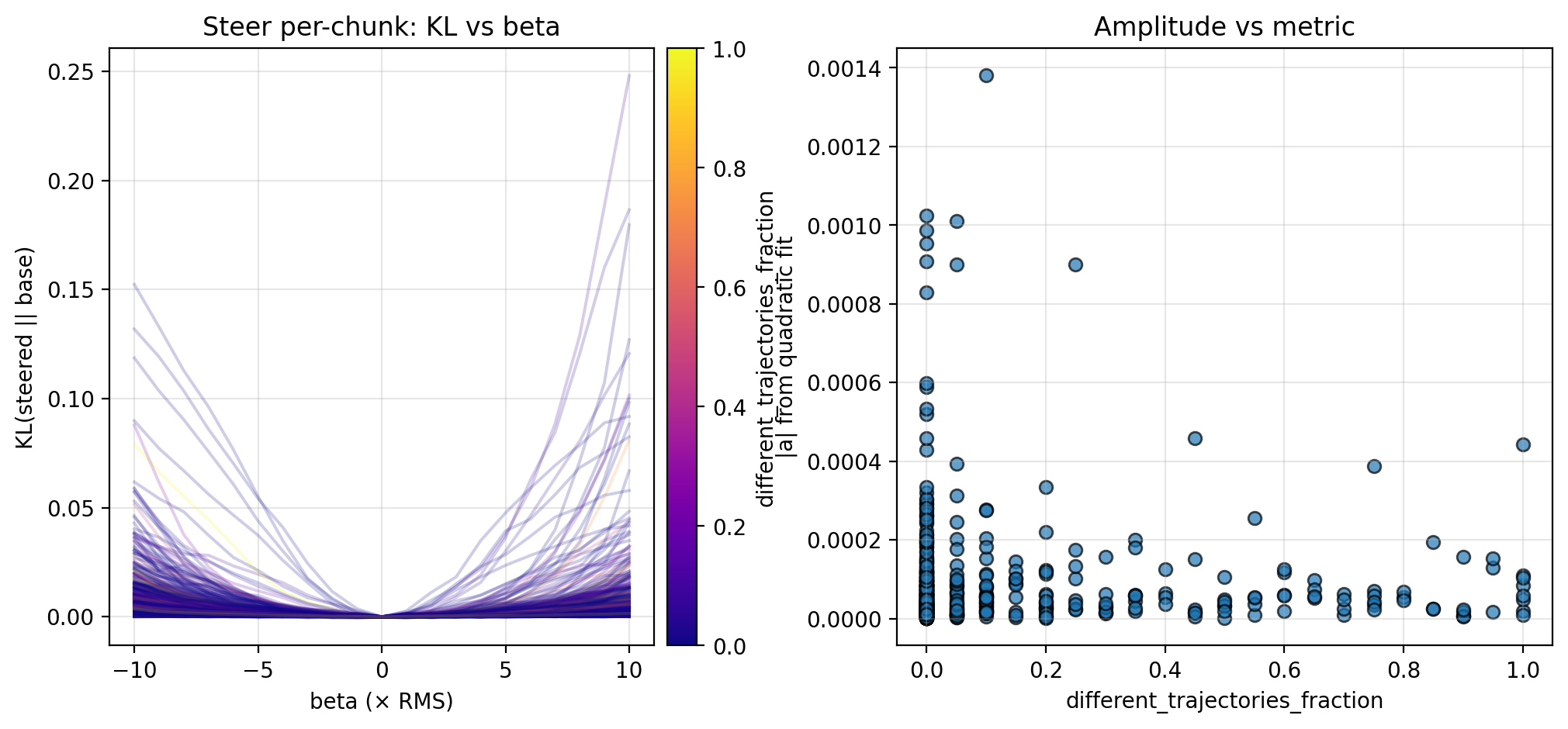
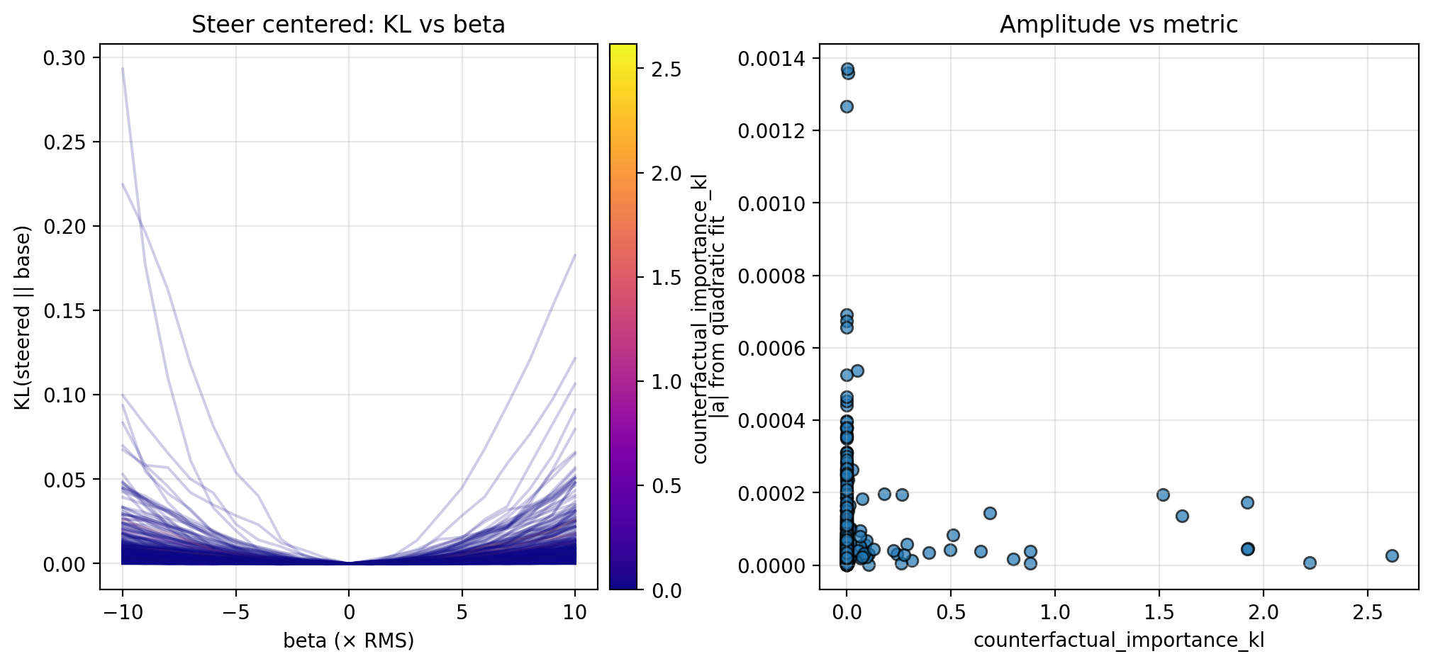
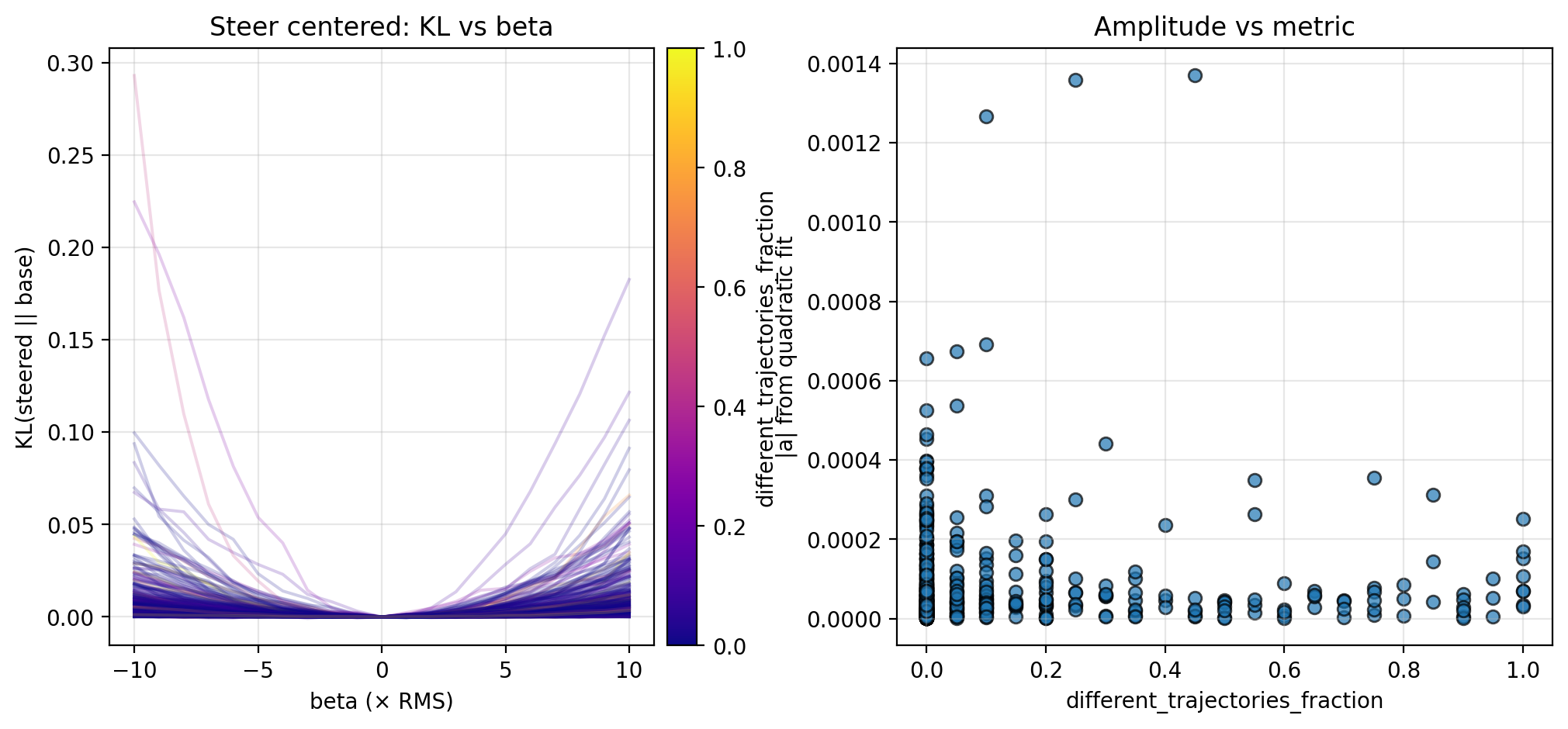
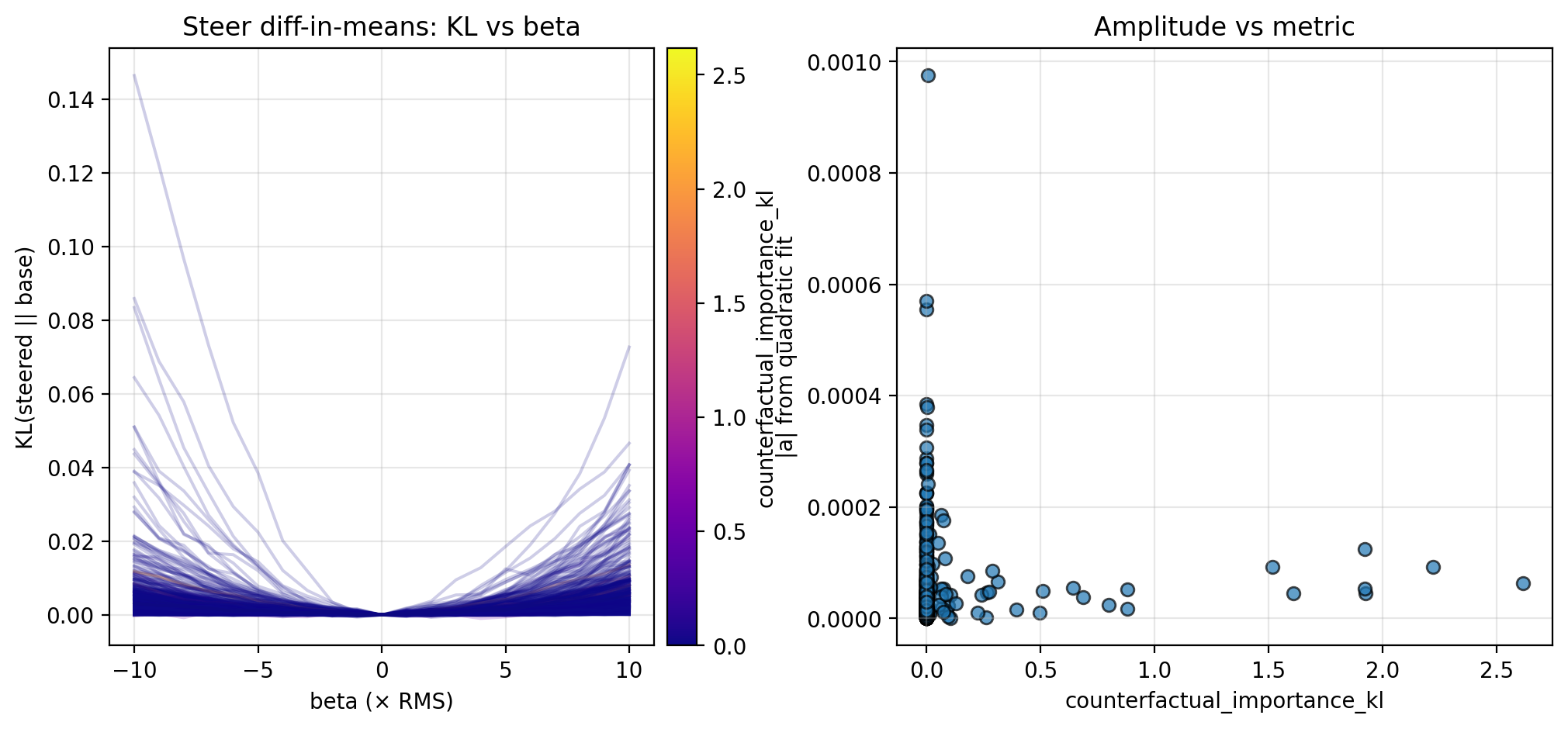
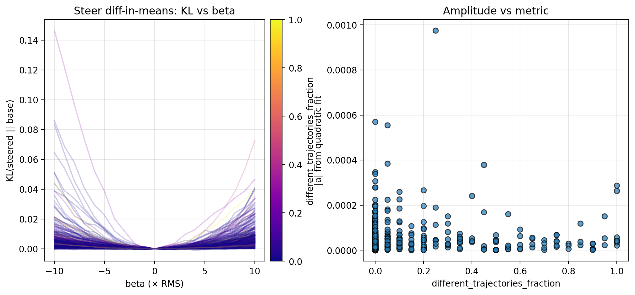
In each case, I measure the KL divergence of the steered activation’s logits (teacher-forced at each token to avoid drift) compared to the base logits across the chunk, and fit a quadratic to the resulting KL curves. For all chunks and examples, I then plot the fitted quadratic amplitude—which serves as a measure of local steepness—against the probabilistic metrics from TA. In this section, I report the results for different trajectories fraction and counterfactual importance; I display the results for counterfactual accuracy in the Appendix, as these are less conclusive.

3.1. Steering Along Privileged Directions

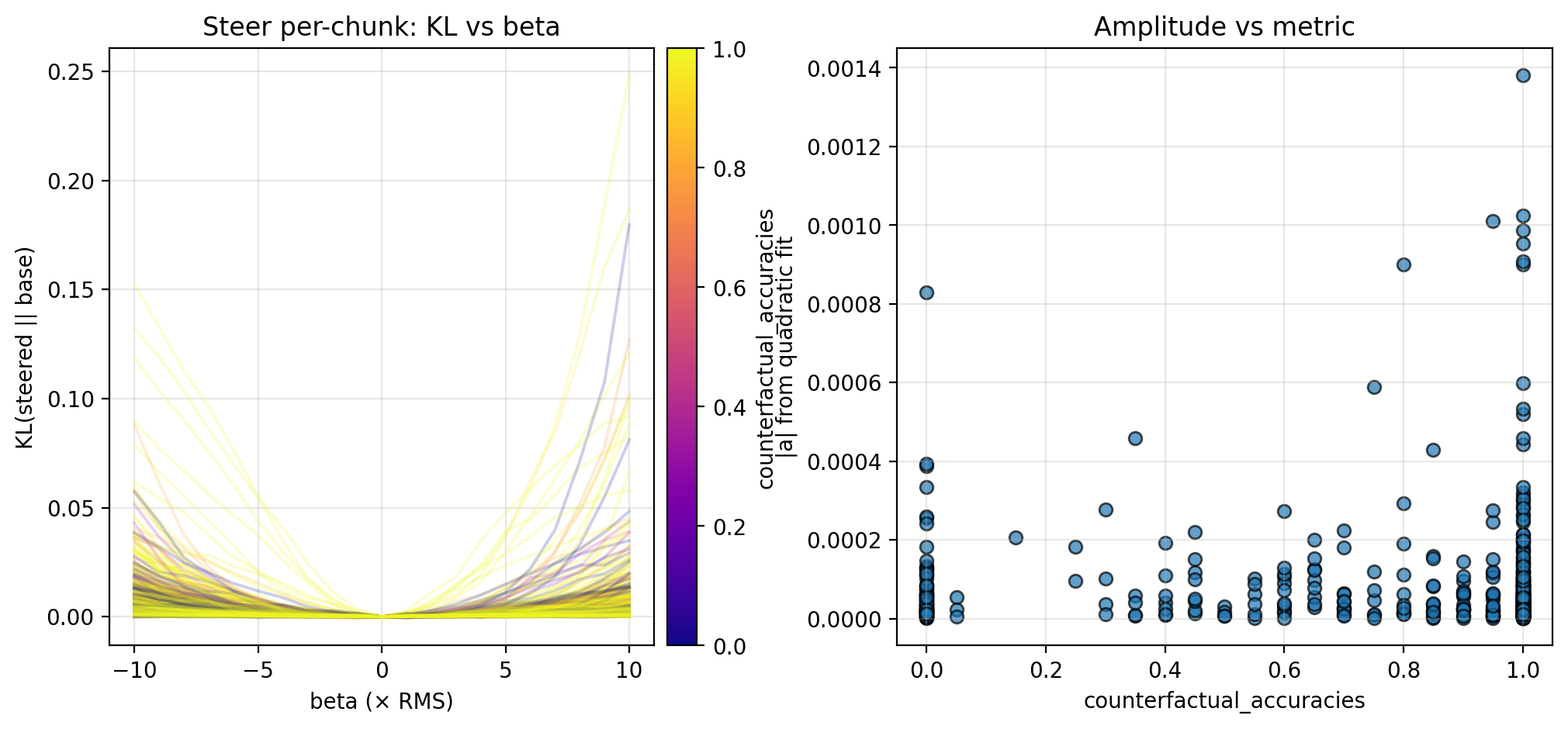
Let $A$ denote the set of chunk activations (collected in Section 2.2), and let $A^+$ and $A^-$ partition $A$ into anchors and non-anchors, respectively (here, I separate $A^+$ from $A^-$ by a counterfactual importance of 0.2, but note that this is a naive approach). I first steer chunk activations ($a \in A$) by a steering vector ($v$) with magnitude $\beta$, so that the activations become $a + \beta v$. In each case, I vary $\beta \in [-10, 10] × \text{RMS}$ (for ~1500 dim. activations, $\text{RMS} \approx 0.026$).

1. Per-chunk, along the chunk activation direction, so $v = a$ (i.e., $a + \beta v = (1 + \beta) \, a$)

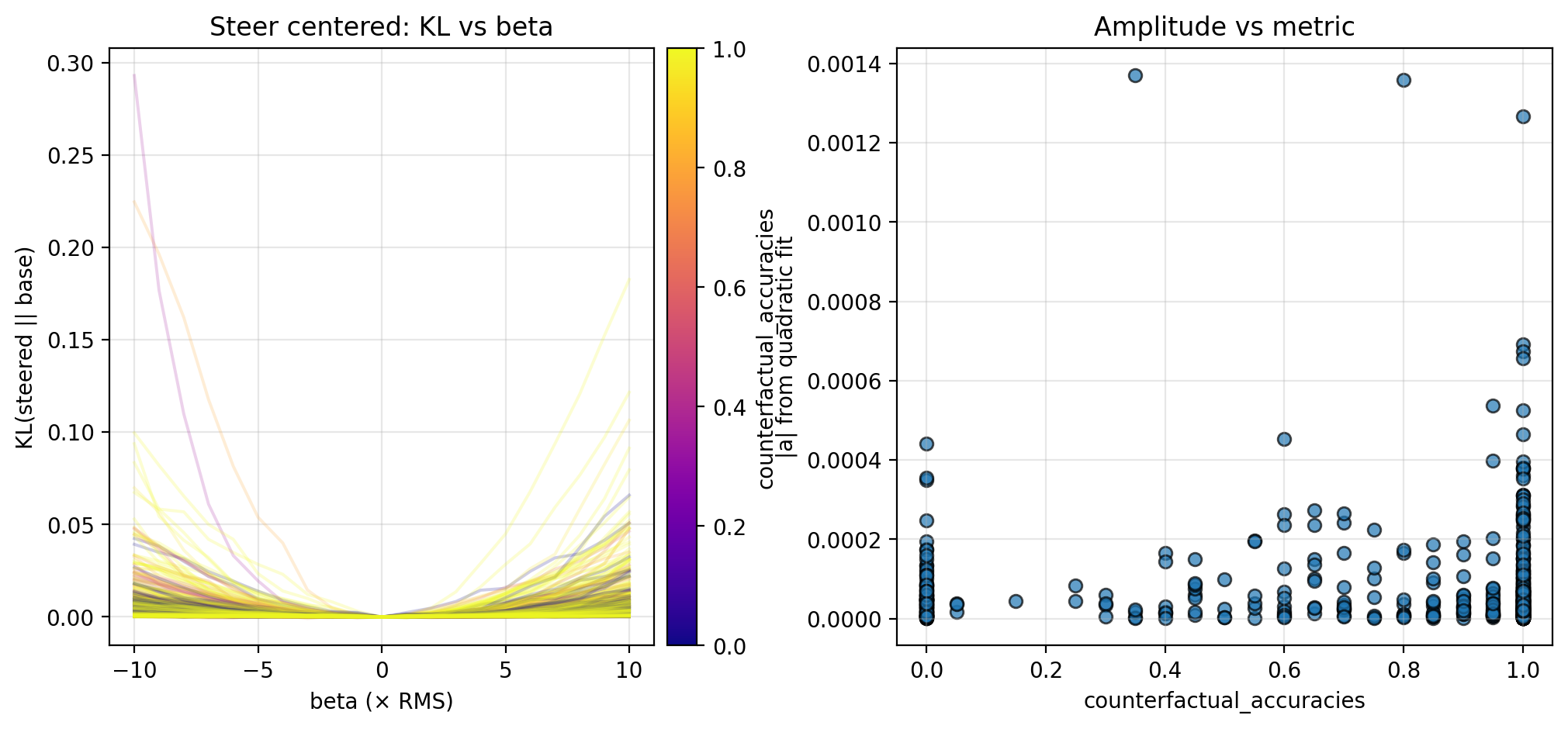
2. Centered, along the mean-subtracted direction, so \(v = a - \frac{1}{|A|}\sum_{a' \in A}(a')\)

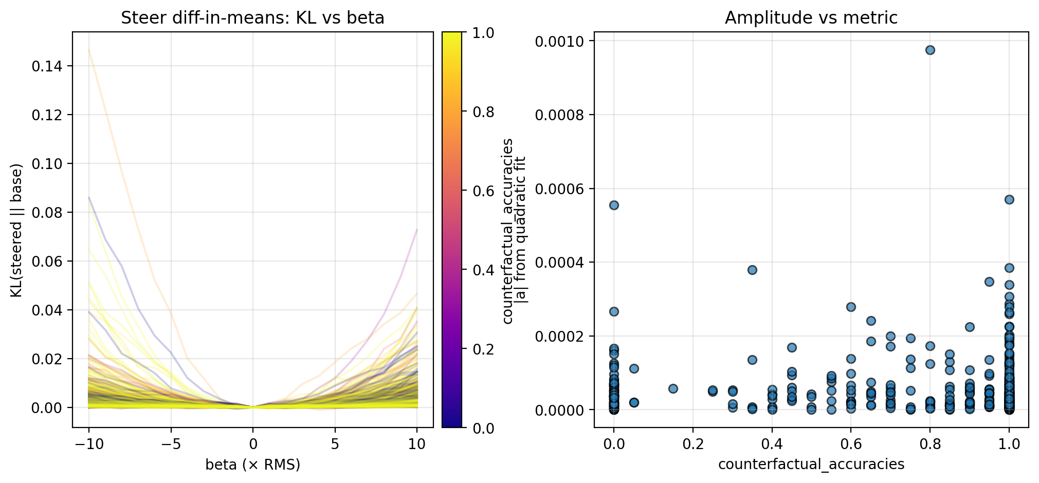
3. Diff-in-means, along the overall “thought anchor direction”, calculated as

\[v = \frac{1}{|A^+|} \sum_{a^+ \in A^+}(a^+) - \frac{1}{|A^-|} \sum_{a^- \in A^-}(a^-)\]

Along each steering direction, I collect KL curves as described above and plot the fitted amplitude versus the different trajectories fraction and counterfactual importance; see the figures below for the KL curves and scatterplots. Though the results are preliminary (discussed further in Section 4.1), these suggest an inverse relationship between the local steepness (along privileged directions) and some logit-level properties of CoT (in particular, different trajectories fraction and counterfactual importance; see Section 4.1 for more discussion).

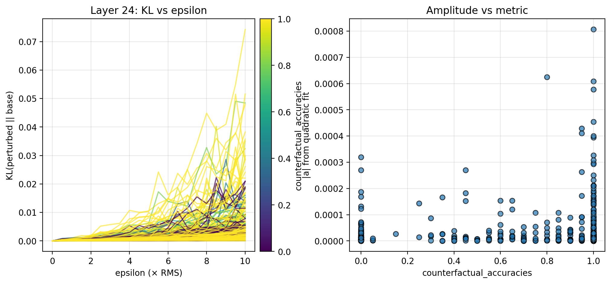
3.2. Perturbing in Random Directions

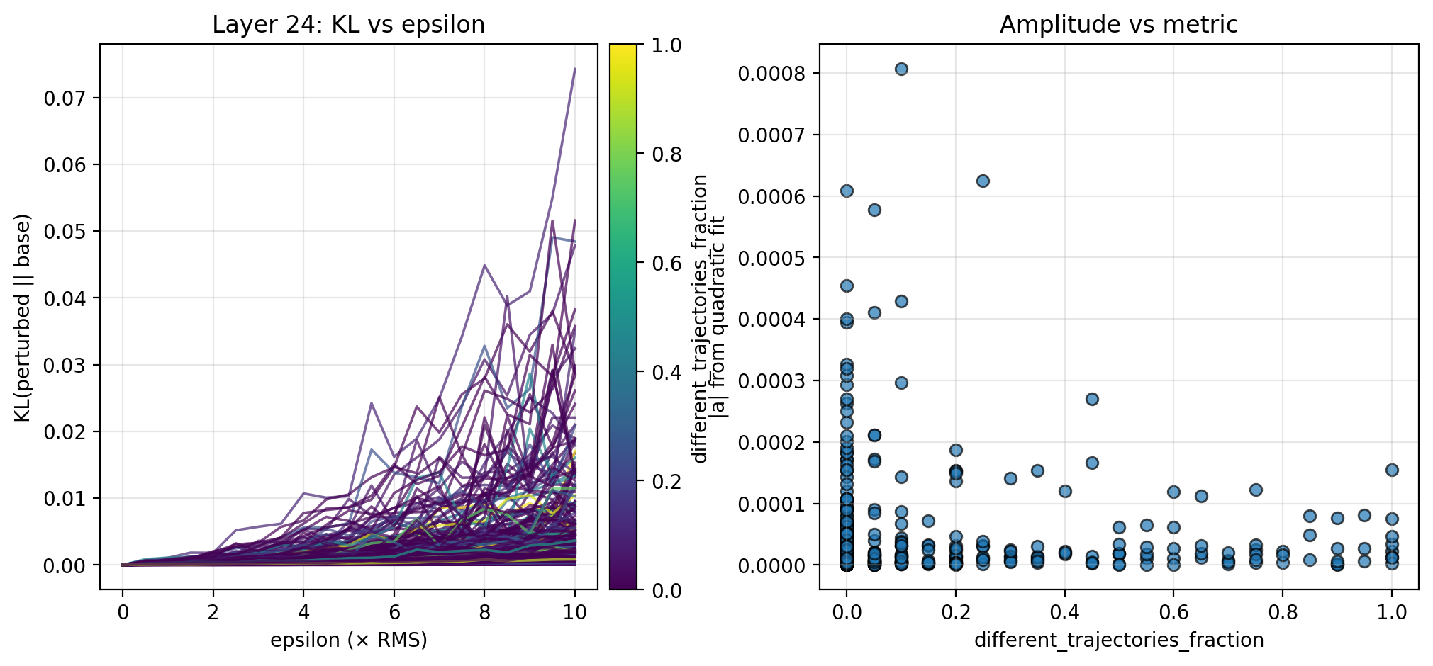
To better understand the overall local steepness around chunk activations, I also perturb in random directions. Specifically, for $\epsilon \in [0, 10] × \text{RMS}$, I perturb $a$ by $a + \epsilon v$, this time choosing $v$ to be a random unit vector in activation space. For each $\epsilon$, I sample 16 directions and average the directional KL divergences. Below, I show the KL curves and scatterplots for isotropic perturbations of chunk activations across the 28 examples. Here too, there is evidence of an inverse relationship between the overall local steepness and both the different trajectories fraction and counterfactual importance.

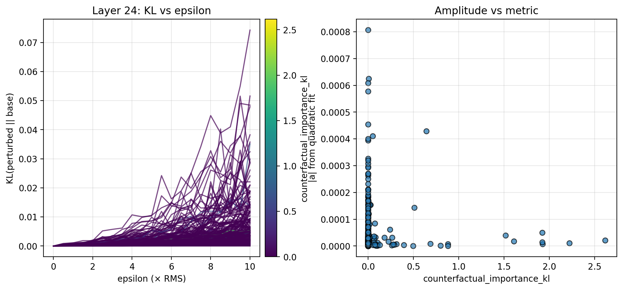
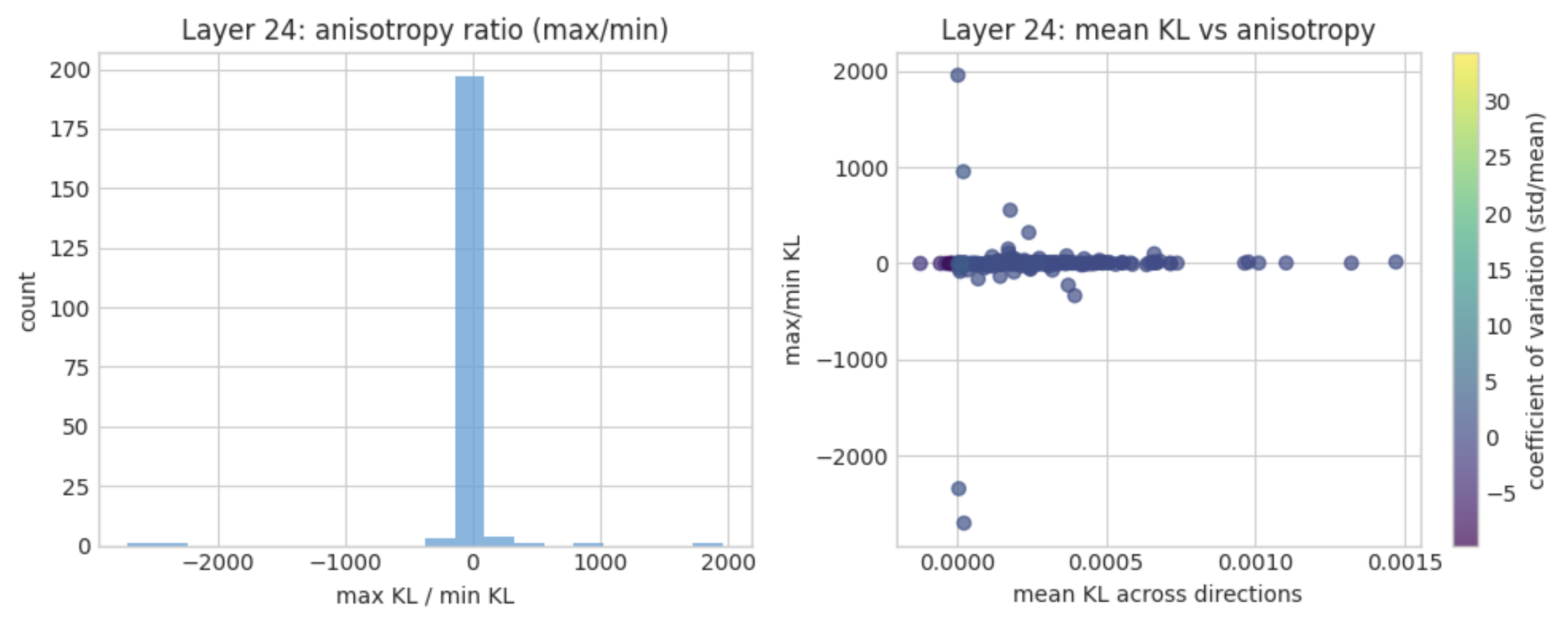
3.3. Local Anisotropy

Do chunk activations lie along steep ridges, or is their local latent space fairly isotropic? To probe this, I fix $\epsilon = \text{RMS}$ and measure the ratio between the maximal and minimal directions of KL divergence. The figure below shows histograms of this ratio across the chunks in a subset of 8 examples (due to time limitations, more below), as well as a scatterplot comparing the ratio with the mean KL (color-coded by the coefficient of variation). Note that negative KL ratios are an artifact of floating-point noise: when the true KL is effectively zero for some random directions, numerical round‑off can produce tiny negative KL estimates, making the ratio negative even though KL is non‑negative in theory. (I plan to fix this in a future blog post, some simple clipping should do the trick; also, sorry that the binning is horrible! As discussed in Section 4.2, these results are especially rough, but this is an interesting direction that warrants further attention.)

4. Discussion

4.1. Relationship between Representations and Logits

The steering and perturbation experiments from Section 3 suggest the possibility that local steepness in latent space is inversely proportional to two logit-level metrics: different trajectories fraction and counterfactual importance. The data here is admittedly preliminary (see Section 4.2 for more detail), but is strengthened by the same pattern observed along multiple steering directions and for random perturbations. If an inverse relationship is indeed true, this suggests that activations in locally flat regions of latent space tend to be more important to downstream computation. This supports recent work observing that latent geometry can have a significant effect on downstream computation (Farzam et al. 2025).

4.2. Limitations

There are many limitations of this small and rather rushed study, which I’ll list in order of which may be most easily addressed:

1. Lack of scale: The results of this post would be much more conclusive by scaling along a few dimensions: (i) model size, (ii) number of examples generated and annotated, (iii) CoT length, and (iv) number of resamples per chunk.

2. Preliminary results: As mentioned throughout, these results are quite preliminary, and are best viewed as an initial indication of a relationship rather than definitive evidence for them. It is certainly very possible that these properties are largely complementary; though visually suggestive, it is less clear if the inverse relationship holds true among the points near the origin, which is the majority. A related notable absence among the results presented here is that I do not robustly fit for the inverse relationship hypothesized between local steepness and some of the logit-level metrics.

3. Naive steering: I test several methods of steering chunk activations: along a few privileged directions, isotropic perturbations, and directional ratios. These methods are fairly naive, especially with respect to the existing geometric structure of the latent space; more sophisticated methods could identify and steer along on-manifold directions. It should be expected that steering along the relevant structure in latent space may reduce some of the noise evident in the figures throughout this study.

4.3. Future Directions

There are a variety of directions from which to extend this work, which I hope to pursue in upcoming posts. Again ordering from least to most ambitious:

1. Addressing limitations: Due to the rushed nature of this post, there is quite a lot of low-hanging fruit; of those explicitly mentioned in Section 4.1, the most interesting would be to collect much more data and fit an inverse function to the scatterplots. (I have already experimented with this; it’s a direction I’m quite excited about pursuing.)

2. Other geometric properties: There are a variety of other local geometric properties that can be studied and connected to the logit-level metrics of TA: local intrinsic dimension, local curvature and shape, et cetera. A good first step in this direction is to improve the analysis of local anisotropy from Section 3.3—these results are (very) rough, but give an idea of the shape of future analysis.

3. Other probabilistic properties: Conversely, there are also a variety of probabilistic properties that can be studied, not least of which are the others in TA.

4. Establishing causation: It would be interesting to move from correlations to causations, as these techniques point the door to other methods than ablation and attribution.

Appendix

Here I include figures from the experiments in Section 3 that I omitted in the main text due. In particular, there appears to be a possible positive correlation with counterfactual accuracy, though these results are notably weaker than counterfactual accuracy and different trajectories fraction. This may be obfuscated by the relatively small amount of data points, or conversely, it is possible that the two are largely complementary and there is little relationship between them.